Python Cheat Sheet
Table of Contents generated with DocToc
- [Up-to-date version: Python Cheat Sheet](#up-to-date-version-python-cheat-sheet) - [Table of Contents](#table-of-contents) - [Numpy¶](#numpy%C2%B6)   - [Create Numpy Array from Python List¶](#create-numpy-array-from-python-list%C2%B6)   - [Create Numpy Array from Built-in Functions¶](#create-numpy-array-from-built-in-functions%C2%B6)   - [Accessing, Deleting and Inserting Elements into NDArrays¶](#accessing-deleting-and-inserting-elements-into-ndarrays%C2%B6)   - [Slicing NDArrays¶](#slicing-ndarrays%C2%B6)   - [Boolean Indexing¶](#boolean-indexing%C2%B6)   - [Set Operations¶](#set-operations%C2%B6)   - [Sorting¶](#sorting%C2%B6) - [Pandas¶](#pandas%C2%B6)   - [Pandas Series¶](#pandas-series%C2%B6)
- [Create¶](#create%C2%B6)
- [Attributes¶](#attributes%C2%B6)
- [Accessing Data¶](#accessing-data%C2%B6)
- [Modify Series¶](#modify-series%C2%B6)
- [Arithmetic Operations¶](#arithmetic-operations%C2%B6)   - [Pandas DataFrames¶](#pandas-dataframes%C2%B6)
- [Create¶](#create%C2%B6-1)
- [Attributes¶](#attributes%C2%B6-1)
- [Accessing Data¶](#accessing-data%C2%B6-1)
  - [Access column(s) by label¶](#access-columns-by-label%C2%B6)
  - [Access column(s) by index¶](#access-columns-by-index%C2%B6)
  - [Access row(s) by label¶](#access-rows-by-label%C2%B6)
  - [Access row(s) by index¶](#access-rows-by-index%C2%B6) - [dtype: object](#dtype-object)
  - [Get N rows from a DF¶](#get-n-rows-from-a-df%C2%B6)
  - [Get N random rows from a DF¶](#get-n-random-rows-from-a-df%C2%B6)
  - [Access element by row and column label¶](#access-element-by-row-and-column-label%C2%B6)
  - [Get all rows where column value satisfies condition¶](#get-all-rows-where-column-value-satisfies-condition%C2%B6)
- [Modify DF¶](#modify-df%C2%B6)
  - [Add column¶](#add-column%C2%B6)
  - [Append columns from a DF to another DF¶](#append-columns-from-a-df-to-another-df%C2%B6)
  - [Insert column at index¶](#insert-column-at-index%C2%B6)
  - [Add column using sum of previous columns values¶](#add-column-using-sum-of-previous-columns-values%C2%B6)
  - [Add rows¶](#add-rows%C2%B6)
  - [Delete column¶](#delete-column%C2%B6)
  - [Delete multiple columns¶](#delete-multiple-columns%C2%B6)
  - [Delete multiple rows¶](#delete-multiple-rows%C2%B6)
  - [Transform values of selected columns¶](#transform-values-of-selected-columns%C2%B6)
- [ Dealing with NaN¶](#dealing-with-nan%C2%B6)
- [Statistical Analysis¶](#statistical-analysis%C2%B6) - [Data Visualisation¶](#data-visualisation%C2%B6)   - [Univariate Data¶](#univariate-data%C2%B6)
- [Categorical data frequency/count as bar chart¶](#categorical-data-frequencycount-as-bar-chart%C2%B6)
- [Categorical data relative frequency as bar chart¶](#categorical-data-relative-frequency-as-bar-chart%C2%B6)
- [Using Barplot to visualise processed data (not already stored as a column value)¶](#using-barplot-to-visualise-processed-data-not-already-stored-as-a-column-value%C2%B6)
- [Numerical data histograms¶](#numerical-data-histograms%C2%B6)   - [Subplots (Stack Plots Horizontally)¶](#subplots-stack-plots-horizontally%C2%B6)   - [Plot Subset of Data (Axis Range Limits)¶](#plot-subset-of-data-axis-range-limits%C2%B6)   - [Axis Transformations (Log Scale)¶](#axis-transformations-log-scale%C2%B6)   - [Bivariate Data¶](#bivariate-data%C2%B6)
- [Pairwise Relationship Between Numerical Columns¶](#pairwise-relationship-between-numerical-columns%C2%B6)
- [Categorical daya grouped-by another label¶](#categorical-daya-grouped-by-another-label%C2%B6) - [Anaconda¶](#anaconda%C2%B6)   - [List envs¶](#list-envs%C2%B6)   - [Activate env¶](#activate-env%C2%B6)   - [Update all packages¶](#update-all-packages%C2%B6)   - [Install package¶](#install-package%C2%B6)   - [specifying package version](#specifying-package-version)   - [Remove package¶](#remove-package%C2%B6)   - [Search package¶](#search-package%C2%B6)   - [List packages¶](#list-packages%C2%B6) - [Jupyter¶](#jupyter%C2%B6)   - [Convert notebook to html¶](#convert-notebook-to-html%C2%B6) - [Other formats](#other-formats) - [https://nbconvert.readthedocs.io/en/latest/usage.html</code></pre>](#httpsnbconvertreadthedocsioenlatestusagehtmlcodepre)   - [Add TOC¶](#add-toc%C2%B6)
layout: post title: “Python cheat sheet” teaser: Python Cheat Sheet - Pandas, Numpy, Data Visualisation Using Matplotlib and Seaborn, Anaconda, Jupyter date: 2020-04-19 00:00:00 +0000 categories: cheat-sheets tags: cheat-sheets permalink: /blog/python-cheat-sheet —
Up-to-date version: Python Cheat Sheet
Table of Contents
- 1 Numpy
- 2 Pandas
- 3 Data Visualisation
- 4 Anaconda
- 5 Jupyter
Numpy
In [2]:
import numpy as np
Create Numpy Array from Python List
In [10]:
x = np.array([1, 2, 3, 4, 5])
print(x)
print(type(x))
print(x.dtype)
print(x.shape)
print(x.size)

x = np.array([[1, 2, 3], [4, 5, 6], [7, 8, 9], [10, 11, 12]])
print(x)
print(type(x))
print(x.dtype)
print(x.shape)
print(x.size)
Create Numpy Array from Built-in Functions
In [32]:
x = np.zeros((3, 4))
print(x)
print(x.dtype)
In [33]:
x = np.ones((3, 4), dtype=int)
print(x)
print(x.dtype)
In [34]:
x = np.full((3, 4), 5)
print(x)
In [35]:
x = np.eye(5, dtype=int)
print(x)
In [36]:
x = np.diag([10, 20, 30, 40])
print(x)
In [37]:
x = np.arange(4, 10)
print(x)
In [41]:
x = np.arange(1, 20, 3)
print(x)
In [42]:
x = np.linspace(1, 20, 3)
print(x)
In [44]:
x = np.arange(20)
print(x)

x = np.reshape(x, (4, 5))
print(x)

x = np.arange(20).reshape(4, 5)
print(x)
In [48]:
# Defaults to range [0, 1)
x = np.random.random((3, 3))
print(x)

x = np.random.randint(4, 10, (3, 3))
print(x)
In [56]:
# mean = 0, std = 0.1
x = np.random.normal(0, 0.1, (5, 5))
print(x)

print(x.mean())
print(x.std())
Accessing, Deleting and Inserting Elements into NDArrays
In [59]:
x = np.array([1, 2, 3, 4, 5])

print(x[0])
print(x[2])
print(x[-1])
print(x[-3])
In [105]:
## Get  diagonal of a 2d array

x = np.arange(25).reshape(5, 5)
print(x)

print(np.diag(x))
print(np.diag(x, k=1))
print(np.diag(x, k=-2))
In [106]:
## Get unique elements of an array

x = np.array([1, 2, 3, 4, 2, 1, 1, 2, 5])
print(np.unique(x))
In [62]:
x = np.arange(1, 10).reshape(3, 3)

print(x)
print(x[0, 0])
print(x[1, 0])
print(x[2, 1])

## Modify element
x[2, 2] = -9
print(x)
In [67]:
## Delete Rows by Index

x = np.arange(9).reshape(3, 3)
print(x)
print(np.delete(x, [0, 2], axis=0))
In [70]:
## Delete Columns by Index

x = np.arange(9).reshape(3, 3)
print(x)
print(np.delete(x, [0, 2], axis=1))
In [72]:
## Append Row

x = np.arange(9).reshape(3, 3)
print(x)
print(np.append(x, [[9, 10, 11]], axis=0))
In [74]:
## Append Column

x = np.arange(9).reshape(3, 3)
print(x)
print(np.append(x, [[9], [10], [11]], axis=1))
In [77]:
## Insert Elements - 1D / Rank 1 Arrays

x = np.array([1, 2, 5, 6, 7, 8, 9, 10])
print(x)
print(np.insert(x, 2, [3, 4]))
In [79]:
## Insert Row at Specified Index - 2D Array

x = np.array([[1, 2, 3], [7, 8, 9]])
print(x)
print(np.insert(x, 1, [4, 5, 6], axis=0))
In [83]:
x = np.array([[1, 2], [4, 5]])
print(x)
print(np.insert(x, 2, [3, 6], axis=1))
print(np.insert(x, 2, 9, axis=1))
In [90]:
## Stack 2 Arrays - Vertically

x = np.array([1, 2])
y = np.array([[3, 4], [5, 6]])
print(f"x=\n{x}")
print(f"y=\n{y}")
print(f"vstack=\n {np.vstack((x, y))}")
In [93]:
## Stack 2 Arrays - Horizontally

x = np.array([[3], [6]])
y = np.array([[1, 2], [4, 5]])
print(f"x=\n{x}")
print(f"y=\n{y}")
print(f"hstack=\n {np.hstack((y, x))}")
Slicing NDArrays
Slicing only creates new "views" on the original array, not new copies of the sliced array. To create a copy, use the copy() method.
In [99]:
x = np.arange(1, 21).reshape(4, 5)
print(x)

print(x[0:2, 0:2])

## Notice the subtle difference between the followig
print(x[:, 0:1])
print(x[:, 0])
Boolean Indexing
In [109]:
x = np.arange(25).reshape(5, 5)
print(x)

print(x[(x > 10) & (x < 17)])
Set Operations
In [110]:
x = np.array([1, 2, 3, 4, 5])
y = np.array([6, 8, 3, 2, 9])

print(np.intersect1d(x, y))
print(np.setdiff1d(x, y))
print(np.union1d(x, y))
Sorting
In [119]:
x = np.random.randint(1, 11, size=(10, ))
print(x)

## Out-of-place sorting
print(f"oop sorted= \n {np.sort(x)}")
print(f"original= \n {x}")

## In-place sorting
x.sort()
print(f"ip sorted= \n {x}")
Pandas
In [121]:
import pandas as pd
Pandas Series
Create
In [128]:
### With default integer indices
groceries = pd.Series(data=[30, 6, 'Foo', 'Bar'])
print(groceries)

### With custom indices
groceries = pd.Series(data=[30, 6, 'Yes', 'No'], index=['egg', 'apples', 'milk', 'bread'])
print(groceries)
Attributes
In [130]:
print(groceries.shape)
print(groceries.ndim)
print(groceries.size)
print(groceries.index)
print(groceries.values)
print('bananas' in groceries)
print('apples' in groceries)
Accessing Data
In [144]:
groceries = pd.Series(data=[30, 6, 'Yes', 'No'], index=['egg', 'apples', 'milk', 'bread'])
print(groceries['egg'])

print('====\n')

## By labels
print(groceries[['egg', 'apples']])
print(groceries.loc[['egg', 'apples']])
print('====\n')

## By index
print(groceries[[0, -1]])
print(groceries.iloc[[0, -1]])
Modify Series
In [145]:
## Change Element Values
groceries = pd.Series(data=[30, 6, 'Yes', 'No'], index=['egg', 'apples', 'milk', 'bread'])
groceries[['egg']] = 31
print(groceries)
In [153]:
## Drop Elements - Out-of-Place
groceries = pd.Series(data=[30, 6, 'Yes', 'No'], index=['egg', 'apples', 'milk', 'bread'])
print(groceries.drop(['apples']))
print(groceries)
In [155]:
## Drop Elements - In-Place
groceries = pd.Series(data=[30, 6, 'Yes', 'No'], index=['egg', 'apples', 'milk', 'bread'])
groceries.drop(['apples'], inplace=True)
print(groceries)
Arithmetic Operations
In [157]:
fruits= pd.Series(data = [10, 6, 3,], index = ['apples', 'oranges', 'bananas'])
fruits + 1
Out[157]:
In [158]:
np.sqrt(fruits)
Out[158]:
In [166]:
fruits[['bananas', 'oranges']] * 10
Out[166]:
Pandas DataFrames
Create
In [171]:
# We create a dictionary of Pandas Series
items = {'Bob' : pd.Series(data = [245, 25, 55]),
         'Alice' : pd.Series(data = [40, 110, 500, 45])}

# We print the type of items to see that it is a dictionary
print(type(items))
shopping_carts = pd.DataFrame(items)
shopping_carts
Out[171]:
In [246]:
## Create DF from csv
# df = pd.read_csv('myfile.csv')
In [172]:
# We create a dictionary of Pandas Series
items = {'Bob' : pd.Series(data = [245, 25, 55], index = ['bike', 'pants', 'watch']),
         'Alice' : pd.Series(data = [40, 110, 500, 45], index = ['book', 'glasses', 'bike', 'pants'])}

# We print the type of items to see that it is a dictionary
print(type(items))
shopping_carts = pd.DataFrame(items)
shopping_carts
Out[172]:
In [178]:
## Creating DF Using Subset of Dict

# We Create a DataFrame that only has selected items for Alice
alice_sel_shopping_cart = pd.DataFrame(items, index = ['glasses', 'bike'], columns = ['Alice'])
alice_sel_shopping_cart
Out[178]:
Attributes
In [174]:
items = {'Bob' : pd.Series(data = [245, 25, 55], index = ['bike', 'pants', 'watch']),
         'Alice' : pd.Series(data = [40, 110, 500, 45], index = ['book', 'glasses', 'bike', 'pants'])}
shopping_carts = pd.DataFrame(items)

shopping_carts.shape
Out[174]:
In [175]:
shopping_carts.ndim
Out[175]:
In [176]:
shopping_carts.columns
Out[176]:
In [177]:
shopping_carts.values
Out[177]:
Accessing Data
In [265]:
items = {'Bob' : pd.Series(data = [245, 25, 55], index = ['bike', 'pants', 'watch']),
         'Alice' : pd.Series(data = [40, 110, 500, 45], index = ['book', 'glasses', 'bike', 'pants']),
         'Charlie': pd.Series(data = [45, 90, 70, 450], index = ['book', 'glasses', 'bike', 'pants'])}

df = pd.DataFrame(items)
df
Out[265]:
Access column(s) by label
In [266]:
df[['Bob', 'Alice']]
Out[266]:
In [256]:
df.loc[:, ['Bob', 'Alice']]
Out[256]:
Access column(s) by index
In [262]:
display(df)
df.iloc[:, [0, 2]]
Out[262]:
Access row(s) by label
In [285]:
df.loc[['bike', 'pants']]
Out[285]:
Access row(s) by index
In [270]:
display(df)
df.iloc[[0, 2]]
Out[270]:
Get N rows from a DF
In [287]:
df[:3]
Out[287]:
Get N random rows from a DF
In [295]:
df.sample(n=2)
Out[295]:
Access element by row and column label
In [188]:
df['Alice']['bike'] # Column label always comes first
Out[188]:
Get all rows where column value satisfies condition
In [259]:
display(df)
df.loc[df['Bob'] > 40]
Out[259]:
Modify DF
In [212]:
items = {'Bob' : pd.Series(data = [245, 25, 55], index = ['bike', 'pants', 'watch']),
         'Alice' : pd.Series(data = [40, 110, 500, 45], index = ['book', 'glasses', 'bike', 'pants']),
         'Charlie': pd.Series(data = [45, 90, 70, 450], index = ['book', 'glasses', 'bike', 'pants'])}

df = pd.DataFrame(items)
df
Out[212]:
Add column
In [201]:
df['Dan'] = [1, 2, 3, 4, 5]
df
Out[201]:
Append columns from a DF to another DF
In [272]:
items = {'Bob' : pd.Series(data = [245, 25, 55], index = ['bike', 'pants', 'watch']),
         'Alice' : pd.Series(data = [40, 110, 500, 45], index = ['book', 'glasses', 'bike', 'pants']),
         'Charlie': pd.Series(data = [45, 90, 70, 450], index = ['book', 'glasses', 'bike', 'pants'])}

df = pd.DataFrame(items)
df

items_new = {'Dan' : pd.Series(data = [1, 2, 3], index = ['bike', 'pants', 'watch']),}
df_new = pd.DataFrame(items_new)
df.join(df_new)
Out[272]:
Insert column at index
In [216]:
items = {'Bob' : pd.Series(data = [245, 25, 55], index = ['bike', 'pants', 'watch']),
         'Alice' : pd.Series(data = [40, 110, 500, 45], index = ['book', 'glasses', 'bike', 'pants']),
         'Charlie': pd.Series(data = [45, 90, 70, 450], index = ['book', 'glasses', 'bike', 'pants'])}

df = pd.DataFrame(items)

df.insert(1, 'Dan', [1, 2, 3, 4, 5])
df
Out[216]:
Add column using sum of previous columns values
In [217]:
df['Total'] = df['Bob'] + df['Alice'] + df['Charlie'] + df['Dan']
df
Out[217]:
Add rows
In [218]:
new_item = {'Bob': 1, 'Alice': 2, 'Charlie': 2}
new_df = pd.DataFrame(new_item, index = ['phones'])
display(new_df)

display(df.append(new_df))
Delete column
In [226]:
items = {'Bob' : pd.Series(data = [245, 25, 55], index = ['bike', 'pants', 'watch']),
         'Alice' : pd.Series(data = [40, 110, 500, 45], index = ['book', 'glasses', 'bike', 'pants']),
         'Charlie': pd.Series(data = [45, 90, 70, 450], index = ['book', 'glasses', 'bike', 'pants'])}

df = pd.DataFrame(items)
display(df)
df.pop('Bob')
display(df)
Delete multiple columns
In [231]:
items = {'Bob' : pd.Series(data = [245, 25, 55], index = ['bike', 'pants', 'watch']),
         'Alice' : pd.Series(data = [40, 110, 500, 45], index = ['book', 'glasses', 'bike', 'pants']),
         'Charlie': pd.Series(data = [45, 90, 70, 450], index = ['book', 'glasses', 'bike', 'pants'])}

df = pd.DataFrame(items)
display(df)

display(df.drop(['Bob', 'Alice'], axis=1)) # 1 = columns
Delete multiple rows
In [232]:
display(df.drop(['watch', 'book'], axis=0)) # axis=0 => row / index
Transform values of selected columns
In [281]:
items = {'Bob' : pd.Series(data = [245, 25, 55], index = ['bike', 'pants', 'watch']),
         'Alice' : pd.Series(data = [40, 110, 500], index = ['bike', 'pants', 'watch']),
         'Charlie': pd.Series(data = [45, 90, 70], index = ['bike', 'pants', 'watch'])}

df = pd.DataFrame(items)
display(df)

columns_to_tranform = ['Bob', 'Charlie']
df[columns_to_tranform] = df[columns_to_tranform].apply(lambda x: x * 100)
display(df)
In [284]:
#### Substitute values in columns of a DF
df.replace([40, 7000], ['Foo', 'Bar'])
Out[284]:
Dealing with NaN
In [240]:
items = {'Bob' : pd.Series(data = [245, 25, 55], index = ['bike', 'pants', 'watch']),
         'Alice' : pd.Series(data = [40, 110, 500, 45], index = ['book', 'glasses', 'bike', 'pants']),
         'Charlie': pd.Series(data = [45, 90, 70, 450, 1], index = ['book', 'glasses', 'bike', 'pants', 'watch'])}

df = pd.DataFrame(items)
display(df)
In [235]:
## Counting NaNs
df.isnull().sum().sum()
Out[235]:
In [237]:
## Counting non-NaNs
df.count().sum()
Out[237]:
In [238]:
## Drop rows with NaNs
display(df.dropna(axis=0))
In [241]:
## Drop columns with NaNs
display(df.dropna(axis=1))
In [242]:
## Replace all NaNs with 0
display(df.fillna(0))
In [244]:
## Forward fill NaNs (value of previous row)
display(df)
display(df.fillna(method='ffill', axis=0)) # Other methods = 'backfill', 'linear'. Axis can be 1
Statistical Analysis
In [247]:
items = {'Bob' : pd.Series(data = [245, 25, 55], index = ['bike', 'pants', 'watch']),
         'Alice' : pd.Series(data = [40, 110, 500], index = ['bike', 'pants', 'watch']),
         'Charlie': pd.Series(data = [45, 90, 70], index = ['bike', 'pants', 'watch'])}

df = pd.DataFrame(items)
display(df)
In [248]:
## Describe statistical information of DF
df.describe()
Out[248]:
In [249]:
df['Bob'].describeribe()
Out[249]:
In [250]:
df.mean()
Out[250]:
In [251]:
df.max()
Out[251]:
Data Visualisation
In [2]:
import pandas as pd
import seaborn as sb

df = pd.read_csv('pokemon.csv')
display(df.head())
Univariate Data
Categorical data frequency/count as bar chart
In [4]:
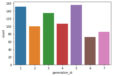
sb.countplot(data = df, x = 'generation_id')
Out[4]:
In [6]:
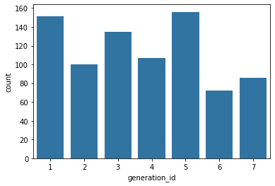
## Single color bars
base_color = sb.color_palette()[0]
sb.countplot(data = df, x = 'generation_id', color = base_color)
Out[6]:
In [10]:
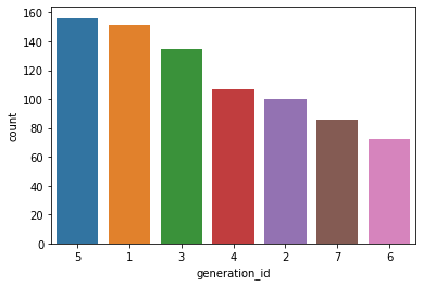
## Sort left to right
gen_order = df['generation_id'].value_counts().index
sb.countplot(data = df, x = 'generation_id', order = gen_order)
Out[10]:
In [32]:
## Rotate x tick labels
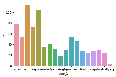
## Without rotation
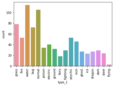
sb.countplot(data = df, x = 'type_1')
Out[32]:
In [33]:
## With rotation
import matplotlib.pyplot as plt

plt.xticks(rotation = 90)

sb.countplot(data = df, x = 'type_1')
Out[33]:
In [36]:
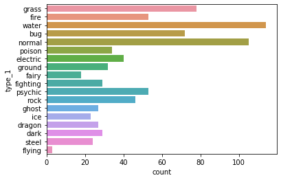
## Plot Y Bars
sb.countplot(data = df, y = 'type_1')
Out[36]:
Categorical data relative frequency as bar chart
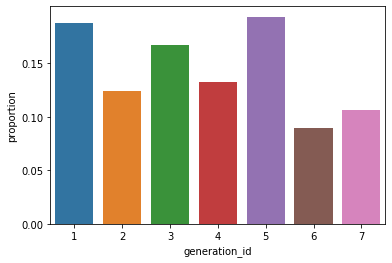
In [51]:
import numpy as np
import matplotlib.pyplot as plt

n_points = df.shape[0]
max_count = df['generation_id'].value_counts().max()
max_percent = max_count / n_points

tick_props = np.arange(0, max_percent,  0.05)
tick_names = ['{:0.2f}'.format(v) for v in tick_props]

sb.countplot(data = df, x = 'generation_id')
plt.yticks(tick_props * n_points, tick_names)
plt.ylabel('proportion')
Out[51]:
Using Barplot to visualise processed data (not already stored as a column value)
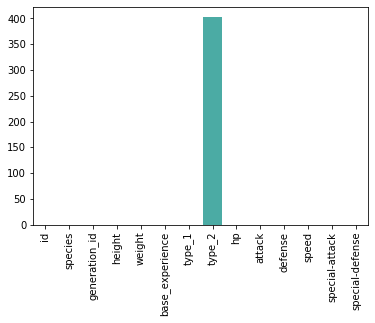
In [55]:
df.isna().sum()
sb.barplot(df.isna().sum().index.values, df.isna().sum())
plt.xticks(rotation = 90)
Out[55]:
Numerical data histograms
In [57]:
df.head()
Out[57]:
In [63]:
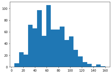
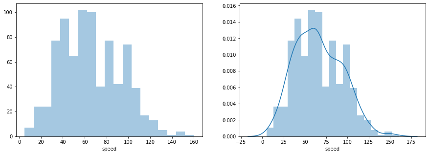
plt.hist(data = df, x = 'speed', bins = 20);
In [64]:
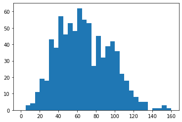
bins = np.arange(0, df['speed'].max()+5, 5)
plt.hist(data = df, x = 'speed', bins = bins);
In [68]:
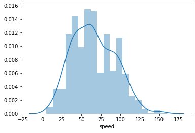
sb.distplot(df['speed']);
In [67]:
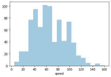
sb.distplot(df['speed'], kde=False);
Subplots (Stack Plots Horizontally)
In [74]:
import matplotlib.pyplot as plt

plt.figure(figsize = [15, 5])

plt.subplot(1, 2, 1)                    # 1 row, 2 cols, subplot 1
sb.distplot(df['speed'], kde=False);

plt.subplot(1, 2, 2)                    # 1 row, 2 cols, subplot 2
sb.distplot(df['speed']);
Plot Subset of Data (Axis Range Limits)
In [79]:
plt.hist(data = df, x = 'height');
In [85]:
plt.hist(data = df, x = 'height');
plt.xlim((0, 2))
Out[85]:
Axis Transformations (Log Scale)
In [87]:
## Original plot (with linear scale)
plt.hist(data = df, x = 'weight');
In [97]:
## Plots with log scales for x-axis
plt.figure(figsize = [15, 5])

plt.subplot(1, 2, 1)
sb.distplot(df['weight'], kde=False)
plt.xscale('log')

plt.subplot(1, 2, 2)
plt.hist(data = df, x = 'weight');
plt.xscale('log')
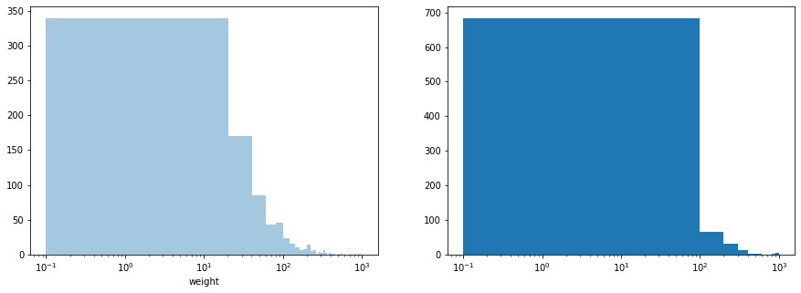
In [98]:
## Changing x range, whilst in log scale to better visualise data distribution
plt.xscale('log')

min = np.log10(df['weight'].min())
max = np.log10(df['weight'].max())
bins = 10 ** np.arange(min, max + 0.1, 0.1)

plt.hist(data = df, x = 'weight', bins = bins);
Bivariate Data
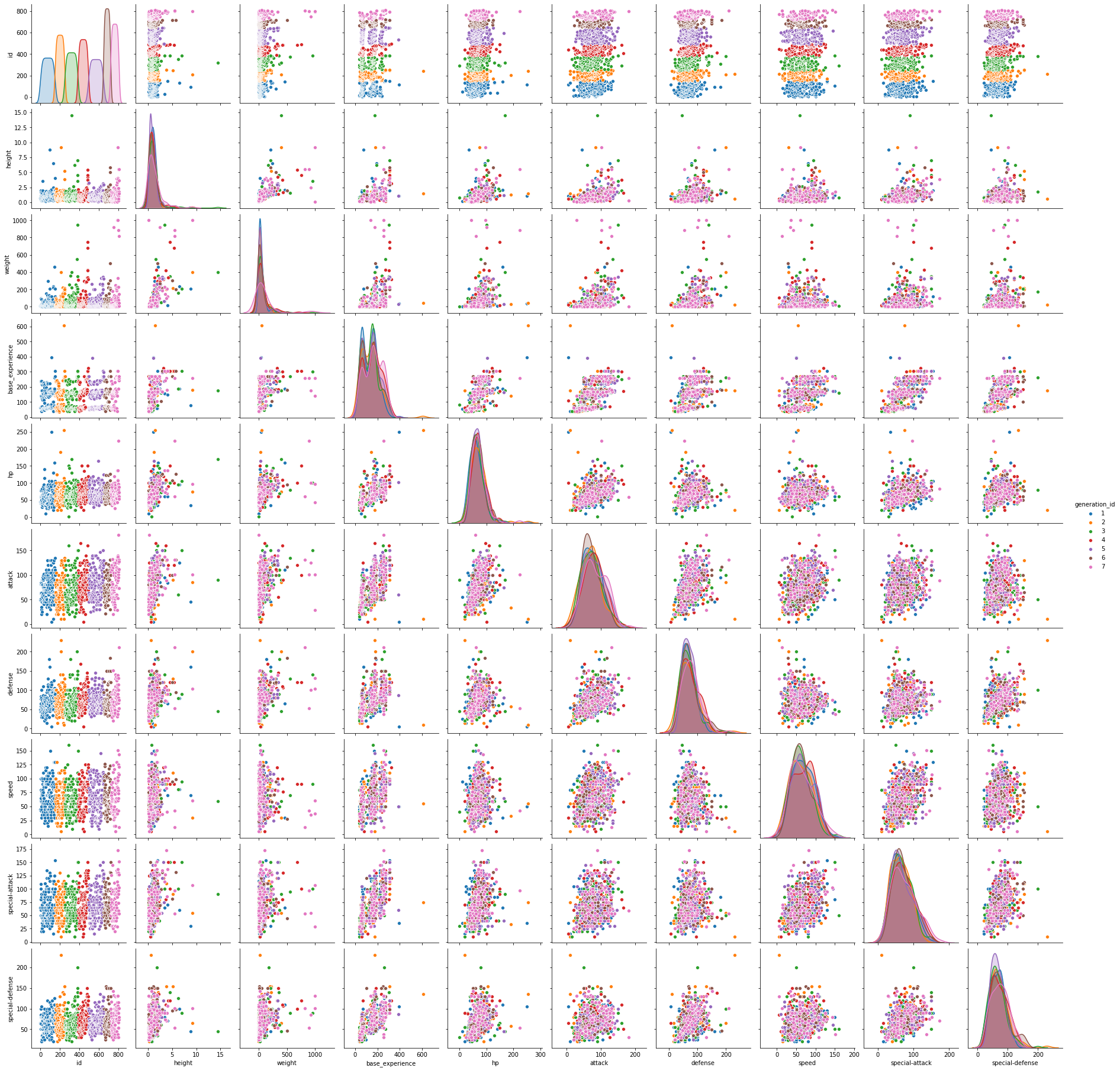
Pairwise Relationship Between Numerical Columns
In [102]:
sb.pairplot(df, hue='generation_id');
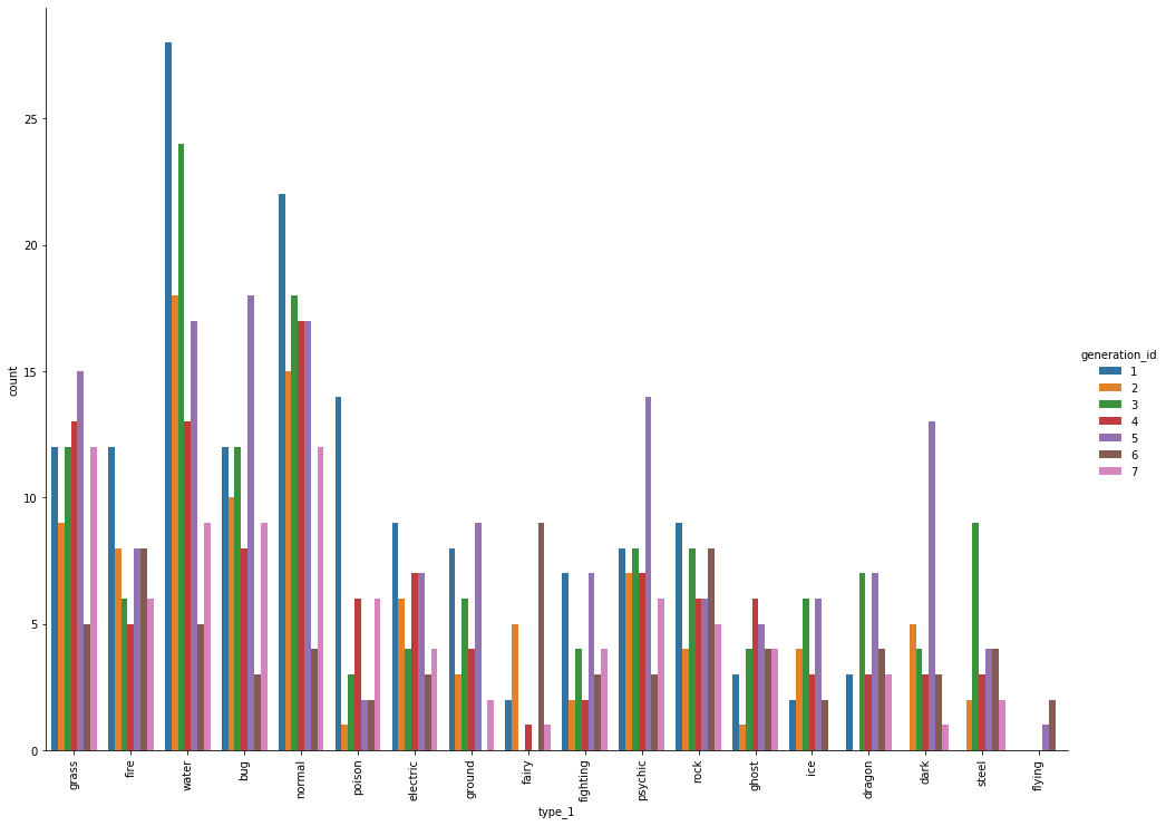
Categorical daya grouped-by another label
In [3]:
df.head()
Out[3]:
In [26]:
import matplotlib.pyplot as plt

chart = sb.catplot(x='type_1', kind='count', hue='generation_id', data=df, height=10, aspect=10/7.5);
plt.xticks(rotation = 90);
Anaconda
List envs
conda info --envsActivate env
conda activate <env_name>Update all packages
conda upgrade -allInstall package
conda install package_name

## specifying package version
conda install numpy=1.10
Remove package
conda remove package_nameSearch package
conda search *search_term*List packages
conda listJupyter
Convert notebook to html
jupyter nbconvert --to html notebook.ipynb

# Other formats
# https://nbconvert.readthedocs.io/en/latest/usage.htmlIn [ ]: